What Is Quantum Measurement? How Observing Qubits Changes Outcomes

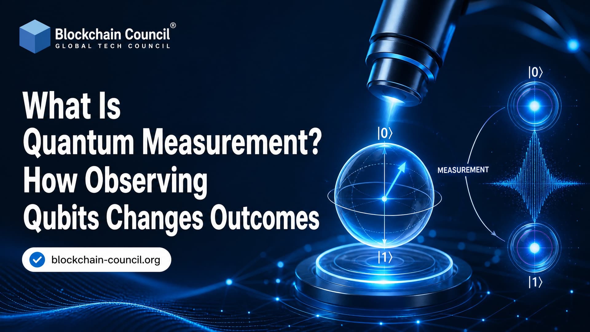
Quantum measurement is the step where a quantum state becomes a classical result you can record, store, or feed into another process. For a qubit, that usually means reading either 0 or 1. The catch is that the act of observing the qubit also changes it. You do not simply peek at a hidden value. You force a quantum state into one of the outcomes allowed by the measurement setup.

This is why measurement sits at the center of quantum computing. It controls what algorithms can output, how error correction works, and how hardware teams judge whether a processor is actually useful.

What Quantum Measurement Means

In standard quantum mechanics, a system is described by a state vector in a Hilbert space. Physical quantities are represented by observables, which are self-adjoint operators. Their eigenvalues are the possible outcomes you can see in an experiment.

For a single qubit, the common computational basis is simple:

• |0>, the classical 0 state
• |1>, the classical 1 state

Before measurement, a qubit can be in a superposition:

|ψ> = α|0> + β|1>

Here, α and β are complex amplitudes. They are not probabilities by themselves. To get the probability of each result, you use the Born rule.

The Born Rule: From Amplitudes to Probabilities

The Born rule says the probability of measuring a result is the squared magnitude of its amplitude. For the qubit above:

• Probability of 0 = |α|²
• Probability of 1 = |β|²
• Normalization rule: |α|² + |β|² = 1

If a qubit is in the equal superposition (|0> + |1>) / √2, measurement in the computational basis gives 0 about half the time and 1 about half the time. Not exactly half in ten shots. Maybe not even in one hundred. But over many repeated preparations, the statistics approach the Born rule prediction.

This point trips up many beginners. You cannot measure one qubit once and recover α and β. A single measurement gives one bit. To estimate the amplitudes, you need many identically prepared qubits and a statistical method such as quantum state tomography.

How Observing a Qubit Changes the Outcome

1. Superposition collapses

When you measure α|0> + β|1> in the computational basis, the result is either 0 or 1. After that, the original superposition is gone. If the outcome was 0, the post-measurement state is |0>. If the outcome was 1, the post-measurement state is |1>.

Measure it again immediately in the same basis and you should get the same answer with probability 1, ignoring hardware noise. That repeatability is a core feature of projective measurement.

2. Information is lost

Measurement does not reveal the full internal state of the qubit. It gives one classical outcome and destroys phase information associated with the original state. This is not a small implementation detail. It shapes algorithm design.

Take phase estimation, amplitude estimation, and variational quantum eigensolvers. All three are built around repeated sampling. They do not assume that one final readout exposes the whole quantum state. It never does.

3. The basis matters

The same qubit can give different statistics depending on the measurement basis. Measuring in the Z basis asks, in effect, whether the qubit is |0> or |1>. Measuring in the X basis asks whether it is |+> or |->, where |+> = (|0> + |1>) / √2 and |-> = (|0> - |1>) / √2.

So yes, the question you ask changes what answer quantum mechanics can give. That is not wordplay. It is the operational heart of qubit measurement.

Projective, Weak, and Mid-Circuit Measurement

Projective measurement

Projective measurement is the model most learners meet first. You choose a basis, the qubit is projected onto one of that basis's eigenstates, and the outcome probability follows the Born rule. Final readout in gate-based quantum circuits usually uses this model.

Weak measurement

Weak measurement extracts partial information through a weaker interaction with the detector. The qubit is disturbed less, but you also learn less per measurement. Repeated weak measurements can strongly affect dynamics. In the quantum Zeno effect, frequent observation can slow or inhibit transitions between states.

That sounds strange until you work with control systems. Measurement is not passive. It is part of the dynamics.

Mid-circuit measurement

Mid-circuit measurement means measuring one or more qubits before the circuit ends, then using the classical result to choose later operations. This is essential for quantum error correction, adaptive algorithms, teleportation, and measurement-based quantum computing.

A practical note: if you test small circuits in Qiskit, watch the bit order in results. Counts strings are displayed with the highest-index classical bit on the left and classical bit 0 on the right. Measuring q into c often appears in the rightmost character. This has caused plenty of false alarms in labs and classrooms.

Measurement in Real Quantum Hardware

In hardware, measurement is not ideal. It has fidelity, latency, leakage, reset cost, and back-action. These numbers matter because a quantum algorithm is only as good as the data you can read from it.

Superconducting qubits

Superconducting transmon systems often use dispersive readout, where the qubit state shifts the response of a microwave resonator. Recent experiments have reported measurement fidelities around 99.8 percent in roughly 200 nanoseconds, with corrected pure measurement fidelity above 99.9 percent after accounting for preparation errors. Other work has shown sub-100 nanosecond readout windows with assignment fidelity near or above 99.7 percent for small groups of qubits.

That said, assignment fidelity is not the whole story. Leakage into non-computational states, energy relaxation during readout, and photon noise can make a system look better on paper than it behaves in a full algorithm. Serious benchmarking measures these effects separately.

Trapped ion qubits

Trapped ions commonly use resonance fluorescence. A bright state scatters photons. A dark state does not, or scatters far fewer. This method can be extremely accurate. Calcium ion optical qubits have achieved average single-shot readout fidelity around 99.99 percent over very large trial counts, with detection times on the order of hundreds of microseconds.

The trade-off is speed. Ion readout is often slower than superconducting readout, but the fidelity can be exceptional. For error correction research, that is a major advantage.

Why Measurement Is Central to Quantum Error Correction

Quantum error correction cannot simply copy qubits and compare backups. The no-cloning theorem blocks that. Instead, codes measure indirect properties called stabilizers or syndromes.

In a surface code, for example, ancilla qubits interact with data qubits and are then measured. The measurement results reveal whether certain error patterns likely occurred, without directly measuring and destroying the encoded logical state. A classical decoder processes the syndrome record and decides what correction to apply.

This is where readout errors become painful. If the syndrome measurement is wrong, the decoder may chase an error that did not happen. Fault-tolerant systems usually need measurement error rates near or below the percent level, depending on the code, noise model, and architecture.

Measurement-Based Quantum Computing

Measurement is not only a final readout step. In measurement-based quantum computing, or MBQC, it drives the computation itself.

The usual model starts with a highly entangled cluster state. Computation then proceeds by measuring individual qubits in carefully chosen bases. Earlier outcomes determine later measurement choices through classical feedforward. In this model, entanglement is prepared first, and measurement patterns implement the logic.

Cluster states are stabilizer states, defined by commuting Pauli operators. Two-dimensional cluster states can support universal quantum computation when measured in suitable bases. This is a serious model, not a teaching trick. Photonic systems, continuous-variable systems, ion traps, and superconducting devices have all explored versions of this approach.

The engineering burden shifts. Instead of executing a long chain of unitary gates directly, you need large resource states, accurate single-qubit measurements, and fast feedforward. If your platform naturally creates entanglement at scale, MBQC can be a good fit. If it cannot, the overhead may be too high.

What This Means for Developers and Security Professionals

If you work in blockchain, cryptography, cybersecurity, or deeptech strategy, quantum measurement has practical consequences:

• Algorithm outputs are samples: A quantum computer usually returns distributions, not single deterministic answers.
• Noise modeling must include readout: Gate error is not enough. Measurement error can dominate small experiments.
• Post-quantum planning needs realism: Breaking cryptographic systems requires not only enough logical qubits, but reliable gates, error correction, and repeated high-fidelity measurements.
• Hybrid systems depend on feedback: Mid-circuit measurement connects quantum processors to classical control loops.

If you want a structured path through this material, Blockchain Council's Certified Quantum Computing Expert™ program covers qubits, quantum gates, algorithms, and measurement concepts in one curriculum. Readers working at the security boundary can pair quantum foundations with blockchain and cybersecurity training.

The Measurement Problem, Briefly

The measurement problem is the gap between smooth Schrödinger evolution and sudden probabilistic collapse. The wavefunction evolves deterministically until measurement, then one definite outcome appears. Standard quantum mechanics treats this as a postulate.

Interpretations disagree on what really happens. Many worlds avoids collapse by branching outcomes. de Broglie Bohm theory adds particle trajectories. Collapse models modify the dynamics. For engineers, the operational rules are enough: prepare states, apply operations, measure many times, compare statistics with the Born rule.

To be blunt, most developers do not need to solve the foundations debate before building useful intuition. But they do need to understand that measurement changes the system, not just the spreadsheet.

Next Step

Build a two-qubit Bell-state circuit, measure both qubits for 1,000 shots, then change the measurement basis on one qubit and compare the counts. That single exercise teaches collapse, correlation, basis choice, and sampling noise better than a page of equations. If you want a guided path after that, study quantum gates, the Born rule, and error correction through the Certified Quantum Computing Expert™ curriculum.